Excel Hack - Lookup Tables Using the vlookup Formula

Here's an Excel hack that I use all the time: lookup tables.

In this previous post I showed how to use Data Validation to create a dropdown list in a cell on a worksheet where I log my fruit consumption.  Imagine I've been logging for a few weeks and have a spreadsheet with dates on it and what fruit I ate on that date.  I now want to log the number of calories each fruit has.  So my Fruit Worksheet looks like this:

Now I could lookup the calorie value of each on the internet and type it into each relevant cell.  But that would be a pain on this sheet as there are repetitions of the same fruit (for example 3 oranges) and will be a real pain as I enter more and more fruit.  Instead I setup a lookup table on my Lookup worksheet; it looks like this:

I then go back to cell C2 (the first calories cell) on my Fruit Worksheet to enter my lookup formula.  I start by typing "=vlookup(" in the cell and I see what's shown below.  Here Excel shows you all the different elements of the formula.

Oh my!  Looks a bit complex.  Let's enter a real life example and then break it down:

So let's match the Excel formula element to what I entered:

• lookup_value becomes B2.  Meaning you're looking up the value from cell B2 (so Kiwi) in the lookup table.
• table_array becomes Lookup!A2:B8 which means our calories lookup table is on a worksheet named "Lookup" in the cell range A2 to B8.  This uses the "!" method to refer to values on a different worksheet, as explained here.  
• col_index becomes 2.  This means, when you've found lookup_value in the first column of the lookup table, you can find the value you're looking up in the second column.  This is useful if you have a lookup table with more than one value to lookup.  e.g. We could have a third column in the lookup table with colour in it and would use 3 as the col_index.
• range_lookup becomes False.  This means don't do an approximate match on the lookup_value, do an exact match.  I always use False to make sure there is an exact match.  I guess you could use True (to get an approximate match) if you were unsure whether the spelling on the target and lookup tables was an exact match.

When I hit return to run the formula you can see the lookup has worked:

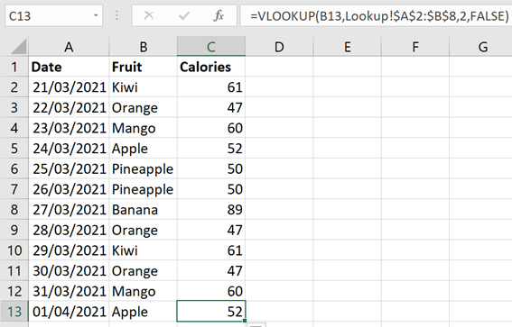
I then tweak the formula to make the lookup table an absolute reference (see here for an explanation).  Here the lookup table cell reference becomes $A$2:$B$8 which means wherever I copy the vlookup formula to on the worksheet, it always refers to the exact same lookup table.

Top tip:  To do this I select cell C2, go to the formula bar, select the cell range and press "F4".  This automatically put the $ signs in.  You can see this below:

With my absolute reference in place I can copy my formula down to all the other Calories column cells and the lookup works just fine!

So that's it for vlookup.  There is also a hlookup formula for where you have a lookup table with your lookup_value in a single row and the values you're looking up below it.  I've never used hlookup as a lookup table such as that shown above just seems "right"!!