Excel Basics - Autofill

Ever noticed the tiny little square on the bottom right of the rectangle that goes around the cell you have selected?   This is called Autofill and it's super useful!  It's circled in the image below:

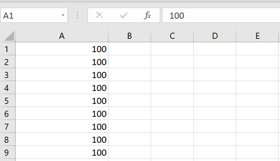
So what does it do?  Hover over it and a little black plus appears.  Click and drag it down (or across) and it acts like copy and paste.  Here's a simple example.  I typed 100 in cell A1, clicked and dragged the Autofill control down to A9 and the value 100 was populated in every cell:

But autofill is cleverer than that.  I put a 1 in cell B1, a 2 in cell B2, selected both cells, clicked the Autofill control and dragged down:

Here autofill has said "hang on a minute, there's a 1 in the first row, a 2 in the second row, I'll continue the sequence".

You can use it to Autofill formulae in cells.  In the image below I put "=A1+B1" in cell C1 then used Autofill to copy it down:

Autofill will also make intelligent decisions if you have text in a cell.  In the example below, I typed "Row 1" in cell D1 then Autofilled down.  Autofill decides to increment the number at the end of the text as you go down:

If you've been watching carefully you'll have seen this little icon appear at the bottom of the set of cells you've been using Autofill on: 

Click on it and you get a bunch of different options for how Autofill works.  The example above is "Fill Series".  If you select "Copy Cells" you get:

...so a straight copy of what you first entered.

If you select "Fill Formatting Only" you get:

...so in this case no obvious formatting.  But if you did have some specific formatting in cell D1 it would be replicated to the cells below.

"Fill Without Formatting" looks to give you the same as "Fill Series" but (assuming you had some obvious formatting in cell D1) it would not be replicated down.

The final "Flash Fill" option is very cool.  Say you have set up a worksheet like this; here you have a name of James Bond actors in column A and you've given Excel as hint as to what you want to do with these values in cells B1 and C1:

Autofill down and you get a default "Copy Cells" view:

But then select "Flash Fill" and you get:

Repeat for the second name and you get:

Clever Excel!

Excel Hack - Getting a Newline in an Excel Cell When Entering Text

Excel is best for numbers but sometimes you find yourself entering lots of text in a cell.  To format the text it's helpful to be able to put in a newline character (aka do a carriage return).  So here's how a bunch of text can look without doing this:

Put in newline characters and hey presto, all a lot easier to read:

So how to do this?  The answer is:

1. Position the cursor where you want the newline, 
2. Hold down the alt key, 
3. Press the return key, 
4. Release the alt key.

Here's where to find the alt key:

...and here's return (also known as Enter):

Hope this is useful.

Excel Hack - Using a "Magic" Apostrophe to Force a Cell to be Text

In Excel you can prefix values in cells with an apostrophe to force Excel to interpret them as text.  Why do this you may ask?

To explain, let's say I want to enter James Bond's telephone number into a spreadsheet.  All I have to do is type 01234007007 (which everyone knows is his number) into a cell, right?  Wrong!  Let's see it in action.  First I type his number (numbers in the UK always start with a 0, that includes MI6 spies):

Because of the leading zero, when I press return, Excel strips the first 0 from what I've typed:

I can get around this by prefixing 007's number with an apostrophe (so a ').  Here we go:

In the image above you can see how the apostrophe is not visible in the cell itself but is in the formula bar at the top right.

Note you also get a little helpful hint warning you there's an apostrophe there.  If you hover over the exclamation mark you get a pop up that says "The number in this cell is formatted as text or preceded by an apostrophe".

So I often use the apostrophe trick for phone numbers or to put formatting in cells that Excel may complain about.  Say I want to write some text in a cell with several sub-points.  You can't do bullet points in a cell so I often prefix lines with a hyphen.  So I type this in:

Hit return and I get:

Oh no!  Because I start with a hyphen, Excel thinks it's a formula with a minus sign, can't interpret the rest of the formula and throws an error.  Put in a magic apostrophe and you get:

Again you can see the apostrophe in the formula bar (top right of the image) but not the cell itself.

Hope that's useful!

Excel Hack - Concatenating (Adding Together) Text in Different Cells

Sometimes in Excel you have values (generally text) in different cells that you want to piece together into a single cell.  In the example below I have a set of fruits and tasty things I want to join together into a single cell:

Lovely old Excel gives us two ways to do this.  The first way, and the one I always remember, is the "&" operator.  In the example below I've already put the formula in cell C1 and am showing the formula structure in cell C2:

The formula simply means "takes what's in cell A2, add a space to it, then add what's in cell B2".

The second way is the "CONCAT" formula.  Here's an example:

Here the CONCAT formula takes a set of cell references and actual strings and joins them all together into a single result.

For (Geek Dad style) fun I can first transpose the column B values to a row (using this method) and then use mixed references (explained here) to create a crazy set of food ideas:

The mixed references in the formula here are used to keep to column A and row 1 as you copy the formula to other cells.  Specifically:

• $A2 - Keep to column A as you copy across columns, allow the row to increment as you copy down.
• B$1 - Allow the column to increment as you copy across, keep the row as 1 as you copy down.

Resulting in:

Comment below if you've used CONCAT or &. 

Excel Basics - Paste Special + Transpose to Turn a Column of Values into A Row

Sometimes in Excel you have values lined up in a single column and you want to get all the values in a single row.  Maybe you want to create a matrix where rows and columns are compared with each other.

Here's an image with made up data to illustrate this:

Let's say I want all the values in column B to actual be across row 1.  So for example "Turnover" goes in cell B1, "Juice" goes in cell C1, "Split" goes in cell D1 and so on.  I could move them one by one but that would be a real pain, especially as the number of values in the column grows.  Instead I use Paste Special and Transpose.  Transpose is the fancy name for changing a row to a column and vice versa.

First, copy the values you want to transpose by selecting them, right clicking and selecting "Copy":

Next select the cell where you want the row of values to be Transposed to. In my case I want the first value in cell B1 so I select that.  I then right click and select "Paste Special...".  The form shown below comes up.  The part of the form I'm interested in is circled:

Tick the "Transpose" box then hit OK.  Lo and behold, what was in the column is now in the row!

You still have your original column of data but you can delete those values and start doing some form of row column comparison!

...and so on!

Note you can also transpose rows to columns.  Comment below if you use this feature!

Excel Hack - Error Checking

A wise person once said "To err is human".  Well Excel sometimes creates errors as well.  Luckily there's a built-in way to check for errors and deal with them.  A common error in computing is dividing by zero.  Here's an example:

Cell C2 shows the formula that's been used.  The "/" part of the formula is how you do divide in Excel and so "=A2/B2" means "take the value in cell A2 and divide it by the value in cell B2".  

You can see how in cell B5 there is the number 0.  In maths (or math for our American friends), a divide by zero is either called infinity or "undefined".  Either way, it can't be computed.  Hence Excel puts an error in a cell where you do a divide by zero, in this case "#DIV/0!".

You can test for a divide by zero using the "ISERROR" formula.  Here's an example:

So the formula "=ISERROR(C2)" simply means "look at the value in cell C2, if it's an error print TRUE, if it's not an error print FALSE".

You can then use an IF formula (see here for an explanation) to test for the error like this:

So the formula above says "look at the value in cell D2.  If it's TRUE print a blank cell, otherwise print the result of the division that was in cell C2.

In the above image I've applied the formula to row 5 where we have the divide by zero and it's come out as blank.  What to set the cell to where there is an error is a design choice.  For example:

• Where there is a divide by zero error you could set the result cell to 0. However if you're also computing something like an average of the column overall you will get a skewed result.  (The average of 3, 3, 9 and 0 is 5.25, the average of 3, 3, 9 and blank is 7).
• You could set the cell to something like "ERROR - FIX ME" then you can search and fix these errors.

What I've shown in the image above is something I often do in Excel to make things more maintainable.  Specifically there is one formula per column (so divide in column C, error check in column D, IF statement in column E).  

You can also chain together more than one formula in a cell like this:

In the above formula in column F we have a error check inside an IF statement.  The way to interpret the formula is:

• So "ISERROR(A2/B2)" to first check if the result is an error.
• If it is an error, make the cell blank.
• If it is not an error, compute A2 / B2 and put it in the cell.

It's up to you how you choose to work.  You can use multiple columns to build up the logic one column at a time or do one big multiple formula entry in a single cell.  I choose the multiple columns option as it makes it easier weeks or months later when you come back to a spreadsheet and try and work out what you actually did!

There's also an "IFERROR" formula that does what I've done above in a single formula.  Additionally there's a bunch of other errors you can check for.  Have a play, see what you can come up with and comment below!

Excel basics - The IF Formula

Occasionally when using Excel you want to analyse the value in a cell and either calculate something differently as a result of the analysis or write something to a cell.  To do this, your friend is the "IF formula".  

Here's an example where I want to analyse the values in column A and write "TRUE" or "FALSE" to column B depending on whether the column A number is positive or negative.  In the image below I show some simple data I've setup in column A and where I've started typing the IF formula in column B to show the different elements of the formula:

Taking each element of the formula in turn:

• logical_test - This is the test you're doing on the values in column A.  So for this formula I'll write "A2>0" meaning "test if A2 is greater than zero".
• value_if_true - This is what to put in column B if the logical_test is true.
• value_if_false - This is what to put in column B if the logical_test is false.

Filling out the first formula I now have:

...and copying the formula to the rest of column B I see:

Note how Excel has used it's clever relative references capability to update the formula as it's copied down to refer to the correct row.

So that's it.  Let me know in the comments below how you use the IF formula.

Excel Hack - Customising the Ribbon

The set of menus menu items across the top of the screen in Excel (and other Office Applications) is called the "Ribbon".  It's the area at the top of the screen that has a set of easy to access menu items for you to use.  Here's a snapshot of the ribbon with key parts picked out:

Here you can see:

• A set of Tabs (Home, Insert, Data etc) which is top level grouping for the ribbon.
• A set of Groups (Clipboard, Font, Alignment etc) which sub-divide the tabs
• Commands (Bold, Italics, Underline etc) which are contained within the groups.  Usually a subset of commonly used things associated with a group.
• A small downward pointing arrow that when clicked opens the main menu for that Group.  So in this example it will open the main Font menu with lots of extra controls over and above those shown in the ribbon group.

I commonly use the strikethrough command (which makes text look like this) but it's not in the Font group on the ribbon.  Hence I need to customise the ribbon.  I start this by right clicking anywhere on the ribbon and selecting "Customize the Ribbon...".  This brings up the form shown below.  It's quite a busy form so I've circled a key control you'll need to use:

I want to create new Group within the Home tab so I simply click the "New Group" button, and a new Group called "New Group (Custom)" appears under "Ideas" in the "Home" tab.  I right click on this, select "Rename", call the new group "Geek Dad", ignore where I can select an image for the group and click "OK".  I then click on my "Geek Dad" group and drag it up under the Font group.  

The form looks like this with my new group circled in blue and another area of the form we'll be dealing with circled in red:

You then click on what I've circled in red and change it to "Commands not in the ribbon".  Scroll down, find the command you want, (in my case strikethrough), click on it and grab it to your new group.  The form now looks like this:

...and the ribbon looks like this:

So go ahead; customise the ribbon to your hearts content for quick access to the controls you frequently use!  Let me know what you get up to in the comments below.

The Curious Power of the PowerPoint Morph Transition

 I've made many a PowerPoint presentation in my time and one feature that always seems to have a wow factor is the Morph Transition.  

Here's a super-simple example in action:

People say "Wow, you got objects to fly around the screen, that must be super complex to do".  Not so; I shall explain how.

So how do you do this?  Super, super easy.  First prepare your "base" slide, the slide that other slides will transition from.  Here's a simple example!

With this slide selected on the slide picker on the left, select the "Transitions" menu and the "Morph" transition as shown below.

Right click on the slide in the slide picker on the left and select "Duplicate Slide" to create a second copy of the slide:

Now edit this second slide by moving and re-sizing the drawing objects:

Put the presentation in slideshow mode, go from the base slide to the next slide and you can see how PowerPoint automatically animates the transition.

This has been an example using made up PowerPoint objects (and ugly ones at that!).  However in my working life I often use this Morph technique to tell a story during technical presentations.  

Say I want to describe a computer system with 4 sub-systems.  I would:

• Prepare a slide with sub-system 1 on it.  The slide has graphic for sub-system 1 and a text description.
• I add a Morph Transition to slide 1 and duplicate it.
• On slide 2 I shrink sub-system 1, show sub-system 2, show how sub-system 1 connects to sub-system 2 and describe sub-system 2.
• Repeat for sub-system 3 on slide 3 and sub-system 4 on slide 4.
• Create slide 5 with all the systems together and a final message.

Real easy but has a big wow-factor.

Excel Hack - Lookup Tables Using the vlookup Formula

Here's an Excel hack that I use all the time: lookup tables.

In this previous post I showed how to use Data Validation to create a dropdown list in a cell on a worksheet where I log my fruit consumption.  Imagine I've been logging for a few weeks and have a spreadsheet with dates on it and what fruit I ate on that date.  I now want to log the number of calories each fruit has.  So my Fruit Worksheet looks like this:

Now I could lookup the calorie value of each on the internet and type it into each relevant cell.  But that would be a pain on this sheet as there are repetitions of the same fruit (for example 3 oranges) and will be a real pain as I enter more and more fruit.  Instead I setup a lookup table on my Lookup worksheet; it looks like this:

I then go back to cell C2 (the first calories cell) on my Fruit Worksheet to enter my lookup formula.  I start by typing "=vlookup(" in the cell and I see what's shown below.  Here Excel shows you all the different elements of the formula.

Oh my!  Looks a bit complex.  Let's enter a real life example and then break it down:

So let's match the Excel formula element to what I entered:

• lookup_value becomes B2.  Meaning you're looking up the value from cell B2 (so Kiwi) in the lookup table.
• table_array becomes Lookup!A2:B8 which means our calories lookup table is on a worksheet named "Lookup" in the cell range A2 to B8.  This uses the "!" method to refer to values on a different worksheet, as explained here.  
• col_index becomes 2.  This means, when you've found lookup_value in the first column of the lookup table, you can find the value you're looking up in the second column.  This is useful if you have a lookup table with more than one value to lookup.  e.g. We could have a third column in the lookup table with colour in it and would use 3 as the col_index.
• range_lookup becomes False.  This means don't do an approximate match on the lookup_value, do an exact match.  I always use False to make sure there is an exact match.  I guess you could use True (to get an approximate match) if you were unsure whether the spelling on the target and lookup tables was an exact match.

When I hit return to run the formula you can see the lookup has worked:

I then tweak the formula to make the lookup table an absolute reference (see here for an explanation).  Here the lookup table cell reference becomes $A$2:$B$8 which means wherever I copy the vlookup formula to on the worksheet, it always refers to the exact same lookup table.

Top tip:  To do this I select cell C2, go to the formula bar, select the cell range and press "F4".  This automatically put the $ signs in.  You can see this below:

With my absolute reference in place I can copy my formula down to all the other Calories column cells and the lookup works just fine!

So that's it for vlookup.  There is also a hlookup formula for where you have a lookup table with your lookup_value in a single row and the values you're looking up below it.  I've never used hlookup as a lookup table such as that shown above just seems "right"!!